Temperature is the dominant abiotic factor determining the distribution of biological diversity on the planet. Extreme temperatures have a profound impact on the performance of all species, including homo sapiens, and ultimately determine where species can continue to thrive (Arnold et al., 2025).—From "Extreme Heat and Agriculture"
Each time the Intergovernmental Panel on Climate Change has issued one of its six assessments of our climate situation over the past 36 years, threats from global warming to the food supply aren't one of the risks that has gotten as much play as they should in headlines or in media reports generally. This isn't because the assessments avoided the subject. On the contrary. From the get-go in 1990, the IPCC authors pointed out that most of the food crops that the bulk of the planet's human population depends on to stay alive would be at risk if our prodigious burning of hydrocarbons continued unabated.
But, for the most part, the discussion early on was full of ifs and whens. Yes, if we stay on the current climate trajectory, then things could get bad, was the widely held perspective. But the when of that happening was viewed as quite far in the future, and would only affect people not yet born. We had time.
The fourth assessment in 2007 marked a turning point. It concluded with stronger data that warming was already affecting some crop systems. An often-cited finding from that report: even modest warming in low latitudes could reduce yields. In 2013-14, the fifth assessment firmed up the assertions of its predecessor with data showing the negative climate impacts on wheat and maize — corn — would be more common than positive ones. There would be serious risks to fisheries and livestock. Undernutrition risks would increase.
The sixth assessment in 2021-23 was the bluntest yet. It noted that climate change had already reduced food and water security for millions of people and had harmed agricultural productivity in many regions. The impact of heat compounded by drought had, it said, led to fisheries declines, crop failures, supply chain disruptions, and labor productivity losses from extreme heat. The assessment pointed out that climate change was doing disproportionate harm in places that had contributed the least to global warming — Africa, Asia, and Latin America in general, as well as Indigenous and low-income populations specifically.
There is a familiar ritual in global governance: catastrophe arrives in increments, institutions issue careful reports, markets shrug, politicians promise frameworks but shelve those reports, and the vulnerable pay. On Earth Day last week, the new World Meteorological Organization and the U.N. Food & Agriculture Organization, jointly released a new report — Extreme Heat and Agriculture that tries to interrupt that ritual by stating what should by now be obvious: The world’s food system is being destabilized by heat. Not someday. Now.
Said FAO Director-General QU Dongyu,“This work highlights how extreme heat is a major risk multiplier, exerting mounting pressure on crops, livestock, fisheries and forests, and on the communities and economies that depend upon them.”
WMO Secretary-General Celeste Saulo said, “Extreme heat is increasingly defining the conditions under which agrifood systems operate. More than simply an isolated climatic hazard, it acts as a compounding risk factor that magnifies existing weaknesses across agricultural systems. Early warnings and climate services like seasonal outlooks are vital to help us adapt to the new reality,”
KEY FINDINGS FROM THE REPORT
• Extreme heat events are becoming more frequent, intense, and prolonged, with major implications for food production systems worldwide.
• Crop yields decline sharply once heat thresholds are crossed — for many staple crops, around 30°C (86°F) during sensitive growth stages.
• Livestock productivity and survival are threatened as heat stress reduces milk yields, fertility, feed intake, and increases mortality.
• Marine heatwaves are disrupting fisheries and aquaculture, with more than 90% of the global ocean experiencing at least one heatwave in 2025.
• Agricultural workers face escalating health and income risks, especially in tropical and subtropical regions where outdoor labor may become unsafe for much of the year.
• Heat acts as a “risk multiplier,” as Dongyu says, worsening drought, wildfire, water scarcity, pest outbreaks, disease spread, and food-price volatility.
Reality is a wheat farmer watching grain heads shrink before harvest. A dairy producer losing output during a heat dome. A fisher hauling emptier nets from overheated waters. A laborer deciding whether to keep working in dangerous temperatures because missing a shift means missing dinner. A dad losing his shit in the produce section when he sees how much grocery prices keep rising.
As noted, many staple crop species begin seeing yield declines above roughly 30°C, with some, of course, more sensitive than others. Heat can interrupt pollination, accelerate maturation before grain development, increase water demand, and invite pests whose geographical ranges expand in warmer conditions. But for livestock, thermal stress commonly begins above 25°C (77°F), and at even lower temperatures for pigs and poultry, which cool themselves poorly. The consequences include reduced eating, slower growth, reduced fertility, reduced milk production, and death in severe episodes. One analysis found milk yields fell half a percent for every hour cows were exposed to high heat stress, with effects lingering for days.
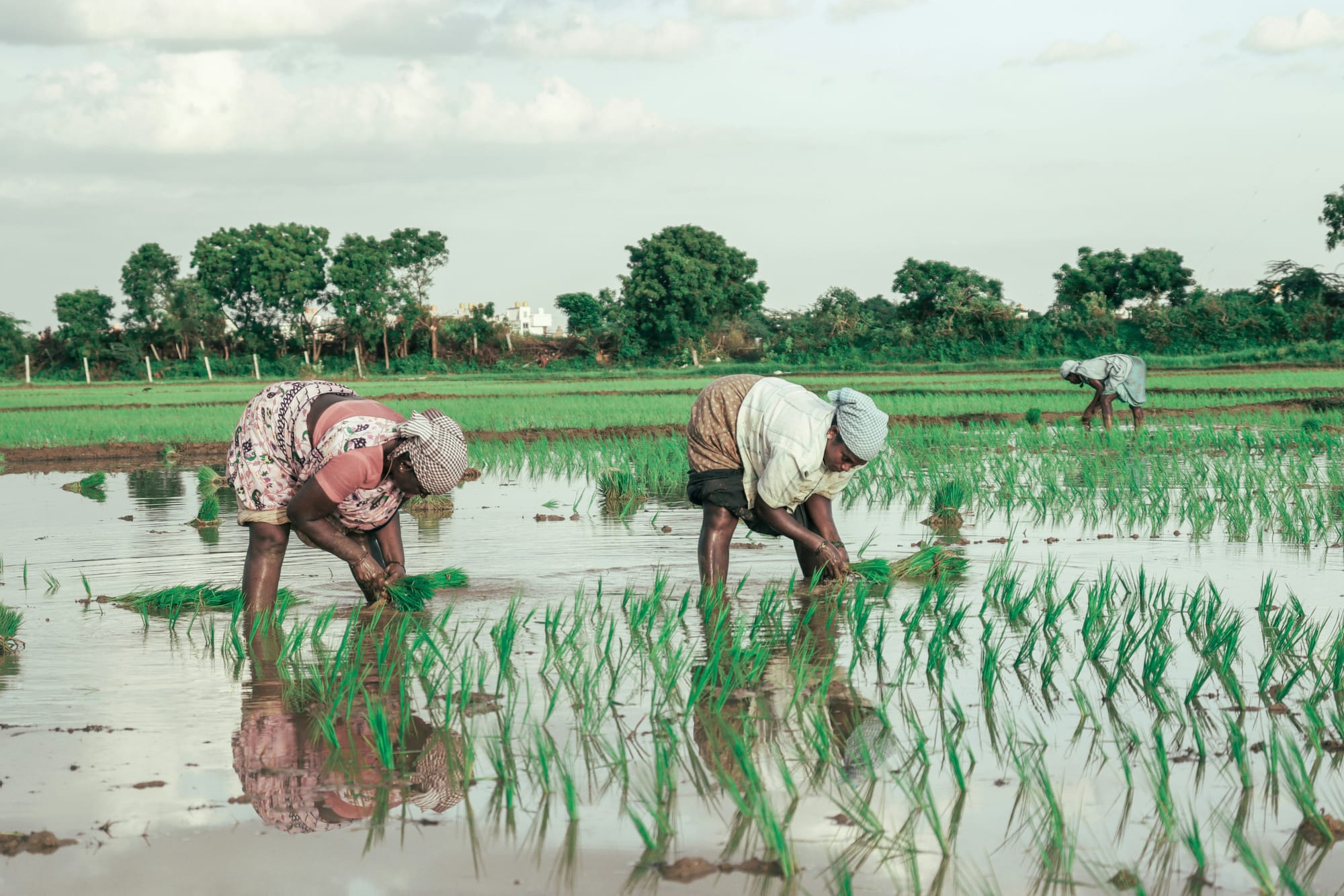
Here's what the report has to say about rice growing amid climate-driven heatwaves in India:
Indian agriculture continues to be vulnerable to weather extremes despite being self-sufficient in grain production. Heat waves cause physiological damage to crops, animals, poultry and fish; reduces water availability; increases demand of water and energy and reduces work efficiency. According to the report Heat Wave 2022: Causes, impacts and way forward for Indian Agriculture [...] March and April 2022 were the warmest months on record in India (Bal et al., 2022). During this period, extreme temperatures were 8 to 10.8°C [14.4°-19.4°F] higher than normal and rainfall was 60 to 99 percent below normal in 10 out of 36 meteorological subdivisions. That year will also be remembered as a classic example of the combined impacts of high temperatures and reduced rainfall felt throughout India's agricultural production systems, specifically in northern and central India. The abonormal increase in maximum and minimum temperatures during 2022 affect crops, fruits, vegetables and lieestock and poultry in over one-third of India's states, including Punjab, Harhana, Rajastahan, Jammu and Kashmir, Himachal Pradesh, Utter Pradesh, Madhyah Pradesh, Bihard and Maharsashtra.
Wheat yields were reduced by 9 to 34 percent. For maize [corn] stunted growth and a fall armyworm attack led to yield reduction of up to 18 percent.
Yield reductions also occurred in chickpeas and multiple fruit crops, with losses of some vegetables as high as 50 percent. Dairy cattle produced less milk, chickens laid fewer eggs and were more likely to die. These effects subsided but lasted longer than the heatwave itself.
Labor, a topic often erased from food discussions, gets some focus in the report, too. Agricultural workers are among the most exposed people on Earth: long hours outdoors, limited protections, and little bargaining power. In some already hot regions, the report asserts that days unsafe for outdoor work may climb to 250 annually before the end of this century. Think about the cruelty embedded in that statistic. The people least responsible for emissions are asked to work inside the blast furnace those emissions built.
That's not the only impact on people. From the report:
In a 2024 report, The Unjust Climate, FAO has assessed the socioeconomic aspects related to extreme weather events in agriculture (FAO, 2024a). The report found that in an average year, poor households lose 5 percent of their total income due to heat stress relative to better-off households. The impacts are even greater for female-headed households who experience annual average income losses of 8 percent due to heat stress relative to male-headed households. Globally, the average annual exposure to heat stress reduces the total incomes of rural female-headed households in low- and middle-income countries by a combined USD 53 billion relative to male-headed households. Over the long-term, a 1°C rise in temperature results in a 54 percent increase in the reliance of poor households on agriculture for income relative to non-poor households. This greater reliance on agriculture increases their exposure to future climate change shocks.
The report includes a lengthy case study of Brazil, where climate stress is colliding with one of the world’s agricultural powerhouses. Brazil is no marginal producer. It exports vast quantities of soybeans, corn, beef, sugar, coffee, and orange juice. When Brazil suffers heat shocks, global markets feel it.
Recent extreme heat episodes, often amplified by drought and shifting rainfall patterns, have damaged Brazilian crop yields and strained livestock production. In key producing regions, excessive heat during flowering and grain-storing periods reduced productivity for soy and corn, while pasture quality declined for cattle. Coffee, especially the arabica varieties grown in southeastern highlands, faces increasing vulnerability because quality and yield depend on relatively stable temperature bands. Push those bands upward, and growers must move upslope, invest heavily, or absorb losses.
Brazil’s case also exposes the political economy of climate risk. The same country that feeds hundreds of millions abroad has millions at home facing food insecurity and volatile prices. When harvests tighten or transport systems are disrupted by drought and heat, domestic consumers can be priced out while exports continue. Field workers harvesting cane, tending cattle, or working logistics networks endure dangerous outdoor temperatures with uneven protections. Heat lowers productivity, increases illness, and raises costs, something that is often unfairly blamed on labor.
Brazil is a warning in plain view. If even a continental-scale farm superpower can be destabilized by heat that is rising in an accelerated fashion, no food system is truly secure.
Secretary-General Saulo is exactly right that extreme heat is increasingly defining the conditions under which agrifood systems operate.” Heat magnifies debt. Heat magnifies water scarcity. Heat magnifies the defects of weak labor law enforcement. Heat magnifies dangers of depending on export monocultures. Heat magnifies hunger.
The authors recommend more climate services, early warning systems, altered planting calendars, resilient breeds, financing tools, insurance, and social protection. Serious and worthwhile measures, to be sure. But there's danger in presenting adaptation as if it were primarily a management challenge rather than a matter deeply entangled with who has political clout.
Who controls the land?
Who controls the seeds?
Who controls the water rights?
Who protects workers?
Who profits from commodity volatility?
Who funds disinformation while emissions rise?
Without candid public answers to those questions and scrutiny of their impacts, crafting new policy is as useful as putting a picket fence around a wildfire.
FAO official Kaveh Zahedi told Reuters that “Extreme heat is rewriting the script on what farmers, fishers, and foresters can grow and when they can grow. In some cases it is even dictating if they can still work.” That sentence should be read in every agriculture ministry on Earth. Because what's being rewritten is far more than the farming calendar. It's the social contract.
As yields fall while input costs rise, farms consolidate, something we've already seen too much of the past half century. As climate makes laboring more perilous, migration increases. As fisheries fail, coastal economies unravel. As prices spike, authoritarian politics feed on grievance and scarcity. Bread has always been political.
SO WHAT SHOULD BE DONE?
Cut emissions fast. No adaptation strategy can keep pace with unchecked warming. Protect workers. Mandatory heat standards, paid breaks, hydration, cooling shelters, and enforcement. Build public resilience. Storage, irrigation efficiency, grids, extension services, and local processing. Democratize seed banks and research. Climate-resilient genetics should not be monopolized. Finance justice. Debt relief and grants for climate-hit nations. Diversify agriculture. Monocultures are profitable in spreadsheets and brittle in heatwaves.
All of that takes money. As the report states, however:
Agriculture adaptation is currently not strongly supported by the financial sector. Agrifood systems received only 4 percent of total climate-related development finance in 2023 (FAO) 2025c). The context framed by these conditions highlights the fact that while technical solutions may exist, their deployment depends on ensuring the presence of supportive socioeconomic policies, financial investment, organizational capacitys and overcoming knowledge deficits and other barriers. In response, fully integrating climate change adaptation planning into traditional planning frameworks will be required to move from tactical to transformative response formulation. This integration will be key to ensuring lasting impacts and a shift away from short-term solutions that are prone to setbacks due to a lack of coherency and sustainability.
For all its descriptive and prescriptive detail, this report should also be read as an indictment. Decades of warnings were met with delay, denial, and profit-taking. For a while now the invoice has been arriving in the form of burned fields, stressed animals, over-drained water resources, dangerous workplaces, and higher food bills.
One of the key projects of addressing the climate crisis is electrification. And on that score, the world is moving at a faster pace than many of the most optimistic analysts ever expected. Still not fast enough, but making steady progress. In agriculture, not so much. The past and present foot-dragging means the impacts on the food supply chain will certainly get worse, perhaps much worse. There is a lot of whistling in the dark about this.